Industrial Motion Control: Complete Guide to Servo, Stepper and Axis Design

Key Takeaway

Industrial motion control is not a motor purchase, it is a matched set of motor, drive, mechanics and feedback. Get the inertia ratio under 10:1, size the drive on RMS torque with 3:1 peak headroom, and size the bus and cables from the same numbers.

1. The Motion Control Stack: Command to Motor Shaft

Every industrial motion control system, from a 3-axis CNC to a 400-tonne forging manipulator, is the same four-layer cascade, and understanding industrial motion control means understanding every layer in that cascade. The layers differ by three to four orders of magnitude in speed and they fail in different ways. Understanding the stack is what lets you diagnose a fault in minutes instead of hours, because the symptom tells you which layer is guilty.

Layer 1: the command and profile generator

Industrial motion control begins long before any current flows. This is the layer where the intent of the operator is converted into a mathematical trajectory, and it is the layer that most often decides whether a machine feels smooth or abrupt. This is where a move becomes a trajectory. The controller takes a target position, a target velocity and a set of limits (maximum velocity, maximum acceleration, maximum jerk) and produces a time-stamped position reference at the servo cycle rate. On a modern drive this lives in the drive itself. On a CNC it lives in the CNC controller, which streams setpoints over the fieldbus. This layer knows nothing about inertia, torque or current. It only knows how to move smoothly and how to stop on a target.

Layer 2: the position loop

In industrial motion control the position loop is the layer the machine builder spends most time on, because this is the loop that determines final position accuracy. The position loop compares the reference position with the measured position and produces a velocity command. It is the slowest loop, typically running at 1 ms inside the drive or at 1 to 10 ms in the controller. Its proportional gain sets how stiff the axis feels and how quickly it rejects a disturbance, but it also sets how much following error you will see during a fast move.

Layer 3: the velocity loop

Industrial motion control tuning usually ends up at the velocity loop, because this is the loop that trades stability against stiffness and it is the fastest loop an engineer can actually influence. The velocity loop compares the velocity command with the measured velocity and produces a current command. It runs at roughly 250 microseconds (4 kHz). This is the loop that determines how stiff the axis feels when you push against it by hand, and its gain is the one that must be reduced when the inertia ratio is too high. The velocity loop is usually the loop that gets mis-tuned, because it responds fastest to a symptom like hunting.

Layer 4: the current loop

The current loop is where industrial motion control stops being a control problem and becomes a power electronics problem. The current loop compares the current command with the measured motor current and produces the switching voltage for the inverter. It runs at 50 to 100 microseconds. Most industrial servo drives hide it completely and set it from the motor’s own parameters, which is the right choice: a badly tuned current loop produces torque ripple and heat that no amount of outer-loop tuning can fix.

How the cascade sets your bandwidth

Each outer loop must be significantly slower than the loop inside it, otherwise the outer loop commands motion the inner loop cannot deliver and the axis rings. The usual rule of thumb is a factor of 3 to 5 between adjacent loops. A 60 Hz current loop allows about 12 to 20 Hz of velocity loop, which allows 2 to 4 Hz of position loop, which allows roughly 0.5 Hz of mechanical bandwidth for the load. That last number is the honest limit on how fast an axis can follow a step without exciting the mechanics.

Loop	Typical cycle	Feedback device	What it controls
Profile generator	1 to 4 ms	None, it is the reference	Shape of the move
Position loop	1 to 10 ms	Encoder or linear scale	Position error to velocity
Velocity loop	250 us	Encoder	Velocity error to current
Current loop	50 to 100 us	Motor model, sometimes encoder	Current to switching voltage

The key structural point of industrial motion control: an open-loop stepper drive has only the current loop. Everything above it is missing, which is exactly why a stepper can lose steps silently and a servo cannot. The comparison is developed in the servo versus stepper selection guide.

2. Servo or Stepper: Making the Selection Properly

Industrial motion control projects fail at this decision more often than at any other industrial motion control decision, because the decision is usually made on price per watt rather than on the physics of the axis. The honest question is not servo or stepper, it is whether the axis can tolerate an error that nobody will be told about.

The stepper case in industrial motion control

There is a place for the stepper in industrial motion control, and it is a good place. The failure is not in choosing a stepper, it is in choosing a stepper for an axis that industrial motion control cannot protect. A stepper converts a commanded number of pulses into an angular position, and it believes it is always exactly there. There is no measurement, so there is no error report. A 1.8 degree stepper at 200 microsteps gives 0.09 degrees of command resolution, which on a 20 mm lead ball screw is 20 x 0.09/360 = 0.005 mm of command resolution. That is excellent, and it is worthless if the motor skipped 40 steps during a rapid move. You would have a 0.10 mm position error and a perfectly healthy drive with no fault code.

The stepper is the right answer when the load is steady, the acceleration is modest, the speed is below about 500 rpm, and the cost of a scrapped part is low. Text labelling, small packaging machines, laser positioning and desktop CNC are all good stepper applications. A closed-loop stepper with an encoder that alarms on lost steps costs roughly 30 to 50 percent more than the open-loop equivalent and removes the failure mode entirely. For new builds, that is the sensible default.

The servo case in industrial motion control

The servo is the default in serious industrial motion control because it turns an open loop into a closed loop, and a closed loop can report its own error. A servo measures rotor position continuously and corrects. It will report a position following error, it will saturate the torque limit instead of losing steps, and it will hold position against an external disturbance. It is the right answer whenever rapid traverse is a significant part of the cycle, whenever the axis must hold against gravity or a cutting force, or whenever a missed position means a damaged tool or a scrapped workpiece.

Criterion	Stepper	Servo
Position error	Undetected if steps are lost	Measured and reported every cycle
Speed range	Poor above 500 rpm, torque falls away	Full constant torque to base speed
Acceleration	Limited by pull-out torque	Limited by motor torque and inertia ratio
Overload	Stalls and loses steps	Current limit, then fault, position held
Efficiency at idle	Poor, holds current to stay on position	Good, current follows load
Cost per axis, Indian market	Rs 8,000 to 40,000 for a small axis	Rs 35,000 to 250,000 depending on power

One frequently missed cost: a stepper holding a vertical axis against gravity dissipates power continuously. A 5.6 Nm NEMA 23 stepper holding 3 Nm at 1.5 A per phase dissipates roughly 10 W of copper loss as heat, and it does so for the entire time the machine is idle. On a machine with a Z axis and a 24-hour shift, that is real money and real cabinet heat. The full torque and holding calculations are worked through in the stepper motor sizing guide.

3. The Axis Design Workflow

An axis design in industrial motion control is a sequence of decisions that each depend on the one before. Skipping to the last decision, choosing the drive first and then looking for a motor that fits, is the single most common cause of an over-specified or badly performing axis.

Step 1: define the motion

Nothing in industrial motion control can be sized until the motion is defined, because every number downstream of this step is a function of it. Write down the stroke, the peak velocity, the acceleration, the move distance, the repeat cycle time, the required positioning accuracy and the repeatability. Get these from the process, not from the machine you already own. A feeding axis that needs 2 mm repeatability needs a very different drive train from a turret indexer that needs 0.01 mm and moves 60 degrees every 8 seconds.

Step 2: work out the force

This is the step where most industrial motion control estimates go wrong, because the process force is often the smallest term and the largest uncertainty. Sum every force on the moving mass: process force, friction, gravity component, and the force to accelerate. For a horizontal axis on recirculating ball rails, the friction term is small, typically a coefficient of 0.01 to 0.02 against normal load, because the balls roll rather than slide.

Step 3: work out the torque at the motor

Converting a force into a torque is where industrial motion control becomes quantitative rather than judgemental. For a lead screw, the torque needed at the screw to produce thrust F is:

T = F x lead / (2 x pi x efficiency)

Take a 400 kg table on an X axis with a 20 mm lead ball screw at 90 percent mechanical efficiency. Friction force is 0.015 x 400 x 9.81 = 58.9 N. Acceleration at 4 m/s^2 needs 400 x 4 = 1600 N. Total thrust at the screw is 1658.9 N. Torque at the screw is 1658.9 x 0.020 / (2 x 3.14159 x 0.90) = 33.18 / 5.6549 = 5.87 Nm.

Step 4: work out the speed

Speed and torque together decide the motor, and industrial motion control needs both, not one or the other. Screw rpm follows from linear speed and lead: N = v x 60 / lead. At 0.5 m/s and a 20 mm lead, N = 0.5 x 60 / 0.020 = 1500 rpm. The motor must be able to deliver its rated torque at that speed, which for a servo means 1500 rpm must be at or below its base speed.

Step 5: work out the power

Power closes the loop between the mechanics and the electrical supply, and it is the number that sizes the cabinet. Mechanical power is P = 2 x pi x N x T / 60. At 1500 rpm and 5.87 Nm, P = 2 x 3.14159 x 1500 x 5.87 / 60 = 922 W. That is mechanical output. Divide by drive efficiency of 0.90 to 0.95 to get electrical input, and multiply by the drive and motor efficiencies to get the supply current.

Step 6: check the inertia ratio

No step in industrial motion control has caused more field problems than this one, and no step has a simpler acceptance criterion. This is where most axes get into trouble, and it deserves its own treatment. Reflect the load inertia back to the motor. For a lead screw, the reflected inertia of a translating mass m through a screw of lead L is:

J_load_at_motor = m x (L / 2 x pi)²

For our 400 kg table at 20 mm lead: J = 400 x (0.020 / 6.28319)² = 400 x 1.0132 x 10^-5 = 4.05 x 10^-3 kg m². Add the screw, coupling and gearbox output inertia, roughly 5 x 10^-5 kg m², for 4.10 x 10^-3 kg m² at the screw. A 750 W servo with a rotor inertia of 5.5 x 10^-5 kg m² gives an inertia ratio of 4.10 x 10^-3 / 5.5 x 10^-5 = 74.5 to 1. That is catastrophic for tuning. The remedies are covered in the inertia ratio and servo oscillation guide.

Step 7: select the feedback device

Choosing where to measure the axis is one of the highest-leverage decisions in industrial motion control and one of the cheapest to get wrong. Encoder on the motor gives you motor position and nothing else. A linear scale on the axis gives you true table position, which is what matters when screw deflection, thermal growth or backlash is a meaningful part of your error budget. This is covered in section 4.

Step 8: select the drive and size the power supply

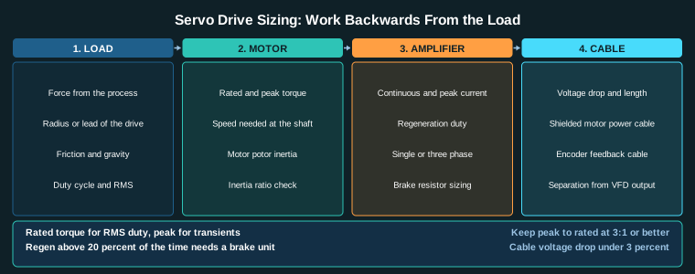
The drive, the supply and the cables are all sized from the same three numbers, and getting them consistent is what makes industrial motion control predictable. The drive is sized on the motor’s continuous RMS current and its peak current. The power supply and the braking resistor are sized on the regeneration side. Cables are sized on the voltage drop and the encoder signal integrity requirement. The servo drive selection and sizing guide works through this in detail.

Step 9: tune, then verify

Industrial motion control is not finished when the axis moves, it is finished when the axis has been measured. Tune from the current loop outward, record the following error for a standard move, and only then sign off. Never sign off an axis on a visual impression of a move.

4. Feedback Devices: Encoders, Scales and Resolvers

The feedback device decides what industrial motion control knows about the world, and therefore what it cannot correct. A drive with only a motor encoder believes the table is exactly where the motor says it is. If the screw stretches 0.04 mm under load, the drive cannot see it and cannot correct it.

Incremental encoders in industrial motion control

The incremental encoder is the default feedback device in industrial motion control because it is inexpensive, rugged and available in every size. Incremental encoders output pulses as the shaft rotates, and the drive counts them. They are cheap, rugged and have no absolute position after power-up, so the drive needs a homing routine or an absolute backup. Output types matter more than most people expect. TTL line-driver (RS-422) differential output is much more noise immune than HTL or TTL single-ended, and on a machine with a 5 kW VFD driving a spindle next to the encoder cable, differential is the minimum sensible choice. Typical resolution for a machine-tool servo encoder is 20 to 24 bits per revolution, which on a 20 bit encoder gives 1024 counts per revolution, or 0.351 degrees of resolution.

Sine-wave encoders

When industrial motion control has to hold a micron over a 500 mm stroke, the encoder is usually the part that has to change first. High-end machine tools use 1Vpp sine-wave encoders with a separate data track for absolute position, offering 23 to 25 bits of resolution and interpolation. The interpolation is a mathematical estimate, so it is only accurate when the machine is at the encoder’s calibrated temperature, which is why the encoder is mounted on the motor housing close to the motor bearings.

Absolute encoders

Absolute feedback has quietly become the default in industrial motion control because it removes an entire class of commissioning risk. A single-turn absolute encoder knows its position within one revolution at power-up, so the drive does not need to home before it can move. A multi-turn absolute encoder also counts revolutions, so it knows the absolute position over many turns. This is standard on modern servo motors and it removes the homing risk entirely, at a cost of roughly 25 to 40 percent more than an incremental encoder of the same class. On a retrofit where the home switch is unreliable, absolute encoders are frequently the best money in the whole project.

Linear scales

A linear scale closes the mechanical loop that an encoder leaves open, and it is the usual answer when industrial motion control needs to measure the load rather than the rotor. A glass or steel linear scale reads position directly at the axis. Optical glass scales resolve to 0.1 to 1 micron and give repeatability of a few hundred nanometres. They cost roughly Rs 25,000 to 150,000 for a 500 mm axis in the Indian market and they add a real constraint: the scale must be mounted rigidly to the same structure as the load and thermally matched to it. A scale bolted to a bracket that is not on the same castings will read the bracket’s error, not the machine’s.

Use a linear scale when the error budget demands better than about 0.02 mm, when the axis is long and the screw deflects, or when thermal growth over a shift is significant. Do not use one on a short, stiff, low-load axis, where it adds cost and installation risk for no measurable gain.

Resolvers

Resolver feedback remains a legitimate choice in industrial motion control where the environment is hostile to optics. Resolvers are sinusoidal encoders with a rotor and a stator, used where an optical encoder would be destroyed by heat, vibration or coolant. They are bulky, need a sine-to-digital converter, and are being displaced by absolute encoders in new machine tools, but they remain the standard in large CNC spindle and turret applications above 100 kW.

Device	Resolution	Knows absolute position	Typical use
Incremental encoder, 1024 ppr	0.35 deg	No	General servo axis, cost sensitive
Absolute single-turn, 20 bit	0.00034 deg	Within one turn	Modern servo motor standard
Absolute multi-turn, 20 bit	0.00034 deg	Yes, over many turns	Turntable, rotary indexer
1 Vpp sine encoder, 24 bit	0.00006 deg	With data track	High precision machining centre
Optical glass scale	0.1 to 1 micron	No, add a reference	Machine tool linear axis

5. Gearing, Couplings and the Inertia Problem

The mechanical transmission between the motor and the load is where the industrial motion control stability budget is usually spent. Every transmission that reduces speed also reduces reflected inertia, which is good, but every transmission that reduces speed with a gear train usually adds backlash and compliance, which is not good. Every transmission adds torsional resonance modes that the controller can excite.

Belts

The simplest way to reduce inertia in industrial motion control is to reduce it with a ratio, and a belt is the cheapest ratio available. A 5 mm pitch synchronous belt with a 30 mm pulley driving a 90 mm pulley gives a 3:1 reduction. The reflected inertia at the motor is the load inertia divided by the ratio squared, so a 3:1 reduction divides the load inertia by 9. Belt drives are not backlash-free: a steel timing belt has essentially no backlash, but a trapezoidal or toothed V-belt has 0.1 to 0.5 mm of stretch and slip under transient load. On a positioning axis, use a steel belt and take the motor-side tension adjustment seriously.

Harmonic drive gearboxes

Nothing has done more to make high inertia axes practical in industrial motion control than the strain wave gearbox. A strain wave gearbox gives 10:1 to 100:1 in a single stage with near zero backlash, a repeatability under one arcminute and a life of 10,000 to 20,000 hours. Reflected inertia falls by the ratio squared, so a 50:1 gearbox divides the load inertia by 2500. This is the standard way to make a high inertia axis tunable. The trade-off is that the gear itself adds inertia at the motor of roughly three to ten times the motor rotor inertia, and adds compliance that creates a torsional resonance mode you must keep the position loop below. Selection is covered in the harmonic drive gearbox selection guide.

Planetary gearboxes

Planetary reduction is the workhorse of industrial motion control where the load is steady and backlash is acceptable. Planetary reducers are cheaper, more efficient (95 to 97 percent) and tolerate shock far better than a harmonic drive, at the cost of 3 to 10 arcminutes of backlash. For a conveyor, a mixer or a winch where the load is steady and backlash does not matter, a planetary box is the right answer. For a positioning axis, it is usually the wrong answer.

Couplings

The coupling is the cheapest component in industrial motion control and the one most often chosen by habit rather than by calculation. The coupling between the motor and the screw must handle the misalignment that the machine build will inevitably have. A bellows or servo coupling is backlash-free and very stiff but only accommodates parallel misalignment of about 0.1 mm. A jaw coupling with an elastomer spider is forgiving but has 0.5 to 3 degrees of torsional deflection, which costs stiffness. A flexible coupling with a spider inserts a low-frequency torsional mode that the position loop can excite, which is one of the classic causes of hunting. The detailed selection is in the shaft coupling guide.

The total inertia budget

Every element in the drive train contributes to the number that decides whether industrial motion control will be stable. Add up the reflected inertia from every element at the motor shaft: the load through the transmission, the transmission’s own output inertia, the coupling, and the screw. That total divided by the motor rotor inertia is the inertia ratio. The number that matters for tuning is the ratio, and the recommended limits are in the next section.

6. Motion Profiles and Jerk Limiting

How the axis moves between two points has as much effect on the machine as how accurately it arrives, and in industrial motion control this is the domain of the profile generator. The profile generator decides the velocity and acceleration history, and it decides how much energy is put into the structure and into the process.

Trapezoidal profile

The trapezoidal profile is the default in almost every industrial motion control system because it is the fastest to execute for a given distance. It accelerates at a constant rate to a constant cruise velocity, then decelerates at the same rate to the target. It is simple, fast to plan and entirely adequate for most conveyor and indexer work. Its weakness is that at the transition from acceleration to cruise, the acceleration changes instantly. That instantaneous change is an infinite jerk, and jerk is what excites machine structure, shakes tooling and produces chatter in a cutting operation.

S-curve profile

The S-curve is the standard answer in industrial motion control wherever the structure, the process or the workpiece is sensitive to a shock load. An S-curve profile limits the rate at which acceleration changes, that is, it limits jerk. The acceleration ramps up over a defined jerk limit, holds, then ramps down. The profile has seven phases: accelerate at jerk limit, accelerate at constant acceleration, decelerate the acceleration, cruise, then the mirror image on the way down. The physical result is that the force transmitted to the machine rises smoothly instead of stepping, which means less structural excitation, less part distortion in a precision operation, and much better behaviour on a long axis with a flexible structure.

The cost of S-curve is time in the acceleration phase, and it is a real cost. For a move where the cruise phase is short, the S-curve profile can take noticeably longer to complete. The full treatment, including the timing arithmetic, is in the S-curve acceleration and jerk limiting guide.

The seven-segment profile

Most industrial motion control drives implement the S-curve as a seven-segment profile, with symmetric segments for a move where the target is far away and a special set of segments for a short move where the axis never reaches cruise velocity. The drive usually exposes three user parameters: maximum velocity, maximum acceleration and maximum jerk, plus a separate acceleration and deceleration limit. Setting all four to sensible values and letting the drive plan the profile is the normal approach.

How jerk limit maps to structure

This is the bridge between a control parameter and the machine, and it is where industrial motion control meets mechanical design. A useful rule is to set the jerk limit so that the frequency content of the acceleration profile stays below the first structural mode of the machine. A trapezoidal profile with infinite jerk theoretically contains all frequencies. A jerk-limited S-curve with a jerk ramp time of 25 ms has its first significant frequency content at about 1/(4 x 0.025) = 10 Hz. If the machine’s first mode is at 40 Hz, you have enormous margin. If the first mode is at 8 Hz, the profile will excite it and you will hear a buzz that moves when you change the acceleration limit.

Position error and following error

If one number defines the health of industrial motion control on an axis, it is the following error. During acceleration, the axis lags the reference because the controller commands a velocity that the motor takes time to reach. This lag is the following error, and it is the single most useful number for diagnosing an axis. The theoretical following error during a constant acceleration is:

e = a x t where e is in metres and t is the velocity loop lag time

With a 2 ms velocity loop lag and an acceleration of 4 m/s^2, e = 4 x 0.002 = 0.008 m = 8 mm. That is enormous, and it is why following error limits exist on precision drives. In practice the velocity loop is faster and the acceleration is lower. With a 0.5 ms lag and 2 m/s^2, e = 0.001 m = 1 mm. If your machine can only hold 5 microns of following error, you need either a much faster velocity loop or a lower acceleration, and the drive tells you which by hitting the following error limit and stopping.

7. Drive Sizing, Power and Regeneration

Sizing a drive is a power-flow calculation, and the most common error in industrial motion control sizing is using peak torque where RMS torque belongs.

RMS torque versus peak torque

Every industrial motion control sizing sheet that is wrong on the motor is wrong here, so this calculation is worth doing properly. The motor rating on the nameplate is the torque the motor can produce continuously without exceeding its temperature rise limit. Peak torque is a short-duration rating, typically 3 times the rated torque for 3 seconds, and you may use it during acceleration but not for a duty cycle that repeats continuously.

Take a machine with a duty cycle: 2 seconds of rapid traverse at 3000 rpm, 1 second of cutting at 500 rpm, 5 seconds of dwell. Compute the RMS torque:

T_rms = sqrt( (T1^2 x t1 + T2^2 x t2) / (t1 + t2) )

Take a machine with a duty cycle: 2 seconds of rapid traverse at 3000 rpm, 1 second of cutting at 500 rpm, 5 seconds of dwell. Compute the RMS torque:

T_rms = sqrt( (T1^2 x t1 + T2^2 x t2) / (t1 + t2) )

Over an 8 second cycle, the rapid traverse needs 18.0 Nm for 2 seconds and the cutting needs 6.0 Nm for 1 second. Dwell contributes no torque. T_rms = sqrt( (18.0^2 x 2 + 6.0^2 x 1) / 3 ) = sqrt( (324 x 2 + 36) / 3 ) = sqrt( 684 / 3 ) = sqrt(228) = 15.10 Nm. That is the torque the drive and motor must be able to deliver continuously. The motor must be rated at 15.10 Nm or more, and the 18.0 Nm during the rapid traverse must be within the peak rating. If the motor is rated 15 Nm with 45 Nm peak, this axis is correctly sized. If someone had sized it on 18.0 Nm alone, they would have oversized it by 19 percent and paid for a bigger drive, a bigger cabinet and a bigger power supply for no benefit.

Power and current

Torque becomes money at this point, and industrial motion control has to be sized in rupees as well as in newton metres. Mechanical power at the shaft is P = 2 x pi x N x T / 60. At 3000 rpm and 18.0 Nm, P = 2 x 3.14159 x 3000 x 18.0 / 60 = 5655 W. The electrical power drawn is P / (motor efficiency x drive efficiency) = 5655 / (0.90 x 0.95) = 6614 W. Current at 415 V three phase is I = P / (1.732 x V x pf x eff). With a power factor near 1 for a servo drive: I = 6614 / (1.732 x 415 x 0.98 x 0.95) = 6614 / 668.8 = 9.89 A. The drive must be rated at least 9.89 A continuous.

Regeneration

Regeneration is the least understood part of industrial motion control sizing and the one that most often produces an oversized cabinet. During deceleration the motor becomes a generator, and the energy has to go somewhere. A drive with a 24 V braking chopper and a brake resistor dissipates it as heat. A drive with a regenerative unit returns it to the DC bus, which then has to be handled by the supply.

The energy returned during deceleration of a rotating mass is E = 0.5 x J x (omega2^2 – omega1^2). For our X axis with J = 4.10 x 10^-3 kg m² decelerating from 1.5 m/s at a 20 mm lead: motor omega = 1.5 / 0.0031831 = 471.2 rad/s. E = 0.5 x 4.10 x 10^-3 x 471.2^2 = 0.5 x 4.10 x 10^-3 x 222,029 = 455.2 J. With a 20 percent duty cycle on the deceleration phase, the average regeneration power is 455.2 / 8 x 0.2 x 8 = 91.0 W, and the peak is 455.2 / (deceleration time). At 4 m/s^2 deceleration from 1.5 m/s, the decel time is 0.375 s, so peak regen power is 455.2 / 0.375 = 1214 W. The brake resistor must handle 1214 W for that short burst. The full method is in the servo drive selection and sizing guide.

Cables and voltage drop

Cable sizing is part of industrial motion control sizing, not a procurement afterthought. Voltage drop limits how far the motor can be from the cabinet. The rule of thumb for a 3-phase motor circuit is that the drop should be under 3 percent of nominal, so under 12.45 V on a 415 V supply. For copper, resistance per metre R = 0.0175 / A (in ohms, for a single conductor of cross-section A in square millimetres), and the loop resistance is twice that for the go and return. Work the numbers from the current and the length before you order the cable, not after the drive trips on undervoltage at full speed.

8. Tuning the Loops

Tuning is not a matter of finding a set of magic numbers, and industrial motion control tuning has a definite order that cannot be skipped. It is a matter of getting each loop to be as fast as the mechanics allow, in the right order, and then stopping.

Start at the current loop

The innermost loop of industrial motion control is the one most often left alone, and that is usually correct. On most industrial servo drives the current loop is set automatically from the motor parameters and you should leave it alone. Verify it only by checking that the motor does not overshoot or ring when you command a small step with no load. If the motor buzzes or the shaft rings at a fixed frequency regardless of the motion, suspect the current loop or the encoder alignment rather than the outer loops.

Then the velocity loop

The velocity loop is the working loop of industrial motion control, the one that a technician will actually adjust in the field. Set the velocity proportional gain to the manufacturer’s recommended value for your motor and load, or start at about half of it. Increase it in 10 to 15 percent steps until the axis starts to buzz, then back off by 30 to 40 percent from that point. That gives you a gain with headroom. Set the velocity integral gain low, to remove the droop in steady-state velocity following, and increase it only until the axis stops complaining at low speed.

Then the position loop

The outer position loop sets how the axis feels to the operator, and it is the loop where industrial motion control tuning most often stops too early. Set the position proportional gain to the manufacturer’s recommendation, then increase it until the axis starts to ring on a fast move, then back off by 30 to 40 percent. On drives with autotune, this whole procedure is done for you, and the autotune result is usually close to optimal. The important step after any autotune is to verify the result with a following error measurement, not to accept it.

Feedforward

Feedforward is the modern part of industrial motion control tuning and the part that most reliably improves an axis without adding gain. Inertia feedforward tells the drive how much torque to command in advance, based on the commanded acceleration and the measured inertia. If the inertia value is correct, inertia feedforward removes almost all of the following error during acceleration, and the result is a stiffer-feeling axis with no increase in gain. This is the single most effective tuning improvement available on a modern drive, and it is free once you have the right inertia number. Velocity feedforward compensates for the velocity loop lag and reduces following error during cruise.

The verification move

Industrial motion control that has not been verified with a measured move is a hypothesis, not a machine. Define a standard move for the axis: a defined distance at a defined velocity with a defined acceleration. Run it and record the peak following error, the time to settle within tolerance, and the repeatability over 10 consecutive moves. Those three numbers are the axis acceptance test, and they should be written down and kept with the machine. The loop hierarchy and the effect of each parameter are explained in the servo tuning guide.

9. Troubleshooting: A Symptom-Led Approach

Industrial motion control faults are mostly diagnosed by elimination, but they are not random, and the symptom narrows the layer almost immediately. The symptom narrows the layer almost immediately, and the layer narrows the cause.

Hunting or buzzing

Hunting is the most common complaint in industrial motion control and the one most often misdiagnosed as a tuning problem. Symptom: the axis oscillates, often at a frequency that does not change when you change the speed. Causes in order of likelihood: encoder signal noise, a loose or poorly shielded encoder cable, a resonance between the drive and the machine structure, excessive velocity gain, or a mechanical looseness somewhere in the drive train. Start by checking the encoder cable and the shield termination. A hunting axis that changes character with speed is more likely a resonance; one that buzzes at a constant frequency regardless of speed is more likely electrical.

Oscillation that grows with load

When an axis is quiet empty and noisy under load, industrial motion control is telling you about inertia or about structure, and the two have different fixes. Symptom: the axis is stable when empty and oscillates when cutting. This is an inertia ratio problem or a structural resonance excited by the load. Check the following error trace during the loaded move. If the oscillation frequency matches the drive’s velocity bandwidth, reduce the velocity gain. If it is fixed, it is structural and you need a filter or a mechanical fix. The full decision tree is in the motion control troubleshooting guide.

Overheating

Heat in industrial motion control is always a current problem, so start with the measured current rather than with the coolant fan. Symptom: the motor or drive overheats during a cycle. Check the motor current in the drive display against the nameplate. If the current is above rated, the load is larger than the calculation said, most often because of a mechanical problem: a dry way, a worn ball screw, a misaligned coupling or a brake that is not releasing fully. If the current is at rated but the temperature still climbs, check the ambient temperature, the cabinet cooling, and whether the motor is correctly derated for it. A servo motor rated 40 degrees C ambient that is mounted next to a hot spindle with no airflow will run 20 to 30 degrees C above its rating.

Position drift or lost position

Position faults in industrial motion control divide cleanly into three cases, and the drive’s own diagnostic tells you which one you have. Symptom: the axis is not where it should be, or the reported position does not match the physical position. First confirm whether the drive is reporting a following error or has lost the encoder reference. If the encoder reference is lost, the problem is the encoder supply, the shield, or the encoder mounting slipping. If the drive reports a large but consistent following error, the axis is being pushed by a mechanical load it cannot resist, or the load is heavier than sized. If the position is right at standstill but drifts during a move, suspect backlash in a belt or gear drive rather than a screw drive.

Faults at specific speeds

A fault that appears at one speed and not at another is the signature of a resonance, and resonance is a mechanical problem inside industrial motion control. Symptom: the axis faults at one particular speed and works at all others. This is almost always a mechanical resonance. The fix is a notch or low-pass filter set in the drive, or a mechanical fix such as changing the coupling type or adding a stiffener. Filtering is the cheap answer and the wrong answer if the resonance amplitude is large enough to be causing fatigue somewhere.

10. The Bus, the Controller and Building the Axis Right

The last layer of industrial motion control is the digital connection between the controller and the drives, and the electrical installation that carries it. This layer has its own failure modes and its own cost.

EtherCAT and Profinet

The fieldbus is what turns a set of independent industrial motion control axes into one coordinated machine. Both are industrial Ethernet protocols with real-time capability, and the difference matters at the level of cycle time and jitter rather than features. EtherCAT uses distributed clocks, giving jitter below 1 microsecond and cycle times down to 250 microseconds, and it processes frames on the fly in the wire, which is why it achieves this on standard 100 Mbps hardware. Profinet IRT uses reserved bandwidth in a standard switched Ethernet network and achieves cycle times of 250 microseconds to 4 ms with jitter in the low tens of microseconds. For a machine with eight axes, EtherCAT is generally the stronger choice; for a plant where the motion bus must share infrastructure with a plant network and where many engineers know Profinet, it is often the more practical one. The comparison is in the EtherCAT versus Profinet guide.

Shielding and grounding

The most common cause of intermittent industrial motion control faults is a grounding and shielding problem, and it is the cheapest thing to fix properly. Use shielded twisted pair for encoder feedback and for fieldbus, terminate the shield at the drive end only with a 360 degree surface mount, and bond every metal part of the machine to a common earth bar with a dedicated strap. Do not route encoder cables parallel to VFD output cables, and if they must cross, cross them at 90 degrees.

Cabinet temperature

Indian shop floors run at 40 to 45 degrees C ambient in summer, and that is a direct derating on every drive in the cabinet. Drives are usually rated to 40 degrees C ambient, so they need derating or a cool cabinet. A drive dissipating roughly 4 percent of its rated power, so a 5 kW drive losing 200 W, needs 200 W of heat removal. A filter fan on a closed cabinet with a heat exchanger is the standard answer.

What a good axis looks like

An axis is correctly built when the numbers are documented, the acceptance test has been run and recorded, the fault behaviour is known, and a technician who did not build it can change a parameter and get the same result. The servo drive sizing guide, the inertia ratio guide and the troubleshooting guide cover the details of each of these steps.

Related Reading

• Industrial Motion Control: Complete Guide to Servo, Stepper and Axis Design
• Servo Drive Selection and Sizing: Power, Regeneration and Cable
• Stepper Motor Sizing: Torque, Speed and Holding Torque Calculations
• Inertia Ratio and Servo Oscillation: Causes, Limits and Fixes
• Servo Tuning: Position, Velocity and Current Loops Explained
• S-Curve Acceleration and Jerk Limiting for Precision Motion
• Harmonic Drive Gearbox Selection: Ratio, Repeatability and Life
• Linear Actuators and Linear Motors: Selection for Machine Axes
• Shaft Couplings for Machine Axes: Rigid, Flexible and Backlash-Free
• Motion Control Troubleshooting: Hunting, Overheating and Oscillation
• EtherCAT vs Profinet for Motion Control: Cycle Time and Cost

Sources

1. Beckhoff Automation, EtherCAT Technology Overview and Cycle Time Specification
2. PI (PROFIBUS & PROFINET International), PROFINET IRT Technology
3. Yaskawa, Sigma-7 Servo Drive Series Operation Manual (loop tuning, inertia ratio)
4. Nidec, Servo Motor Sizing and Motor Selection Guide
5. ISO 9283, Machine tools: Test conditions for positioning accuracy and repeatability of numerically controlled axes

Key Takeaways

• Industrial motion control is a four-layer cascade: profile generator, position loop, velocity loop, current loop. Each outer loop must be 3 to 5 times slower than the one inside it.
• A stepper has no feedback, so a lost step is an undetected position error. On any axis where a scrapped part is expensive, use a closed-loop drive or a servo.
• Size the motor on RMS torque over the real duty cycle, not on the peak torque of the fastest move. The difference is typically 15 to 25 percent.
• Keep the inertia ratio below 10:1 for general work and below 5:1 for high acceleration. Above 30:1 no amount of gain tuning will produce a stable axis.
• Verify every axis with a standard move and record the peak following error, the settling time and the repeatability over 10 runs. An unverified axis is not commissioned.