

Key Takeaway: PLC scan time — the total time your controller takes to read inputs, run the program, update outputs and do housekeeping each cycle — defines how fast the machine can react, and keeping it tight and low-jitter is the difference between a machine that feels responsive and one that rejects parts or overshoots.
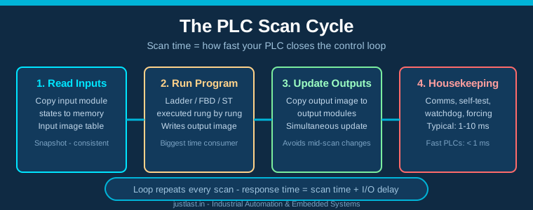
Table of Contents
1. What PLC Scan Time Actually Is
A programmable logic controller does not run instructions continuously the way a PC does. It runs in fixed loops called scan cycles, and PLC scan time is simply the duration of one complete cycle: read all inputs, execute the entire user program, write all outputs, and do internal housekeeping. Screw up your understanding of this rhythm and you will misdiagnose machine faults for years.
Why does the scan matter so much? Because the PLC is a snapshot machine. Every cycle it takes a consistent picture of the input states, executes the logic against that picture, and only then pushes the result to the outputs. That design guarantees predictable, repeatable behaviour — but it also means an input that changes in the middle of a scan is not seen until the next one, and an output decision is always at least one scan old by the time it reaches the actuator. The practical consequence: a machine’s reaction delay is roughly one scan time plus the I/O hardware delays, and everything you do inside the program — every rung, every function block, every communication call — adds directly to that delay.
Typical scan times for modern PLCs range from well under a millisecond for a small micro-PLC running simple logic, to a few milliseconds on a mid-range controller with a big program. The range that matters is not the number itself so much as what your application needs: a slow packaging line tolerates 5 ms easily; a servo axis being synchronised cannot.
2. The Four Stages of Every Scan Cycle
Every scan cycle, regardless of PLC brand, walks the same four stages:
- Read inputs. The PLC copies the states of all digital and analog input modules into an input image table in memory. The program never reads the physical inputs directly; it reads this snapshot. This is what makes the scan consistent — every rung sees the same input values.
- Execute the program. The CPU runs the logic (ladder, FBD, structured text) rung by rung, left to right and top to bottom, updating an output image table in memory along the way. This is usually the largest component of scan time, and it grows with program size and complexity.
- Update outputs. At the end of the program, the output image is copied to the physical output modules together. Outputs never change in the middle of program execution, so a coil that is on at cycle end and a coil that turned on earlier both change at the same moment.
- Housekeeping. Communication (sending process data to SCADA or other PLCs), self-diagnostics, watchdog resets and force handling all happen here. Communication tasks in particular can add a significant slice to scan time on busy networks.
This four-stage model matters when you debug: if an output seems to “stick” for one extra cycle, check whether you are describing a physical output delay or a scan-latency effect — they feel identical to an operator and only the timing logic on a scope will tell them apart.
3. Scan Time vs Response Time
Response time is the interval between a real-world event (a limit switch closes) and the real-world action (a valve opens). It is not the same as scan time, and the difference is where production problems hide. Response time = input filtering time + input module update delay + scan time up to the point the logic sees the input + program execution + output module update delay + actuator response.
Worst-case response is important: an event that happens just after the input read stage waits nearly a full scan before the logic even sees it, so worst-case response is roughly input delay + full scan time + output delay. If your safety or quality logic depends on catching an event, always design for the worst case, not the average. A shield installed to catch a fault “usually in time” will fail on the unlucky cycle — and the unlucky cycle always arrives.
Industrial Ethernet protocols such as PROFINET and EtherCAT exist largely to shrink this latency while exchanging more data — a fieldbus network whose cycle time is 1 ms can synchronise drives and sensors far better than a legacy serial bus polled at 10 ms. When you are choosing between those protocols, response time is one of the first questions to ask the vendor.
4. Jitter: The Hidden Killer of Synchronised Motion
Average scan time tells you how fast the PLC runs on a good day. Jitter — the variation in scan time from cycle to cycle — tells you how truthful the average is, and for serious applications jitter matters more. A controller that averages 2 ms but occasionally stalls to 6 ms to service a communication task will corrupt time-sensitive logic: pulse trains become uneven, analog loops churn, and anything synchronised across devices drifts.
The usual jitter sources are communication processing (performing large block transfers on the same CPU that runs the logic), diagnostic and logging calls, and certain fieldbus masters that inject their own timing into the scan. This is why motion-capable PLCs and servo systems offload the timing-critical control to dedicated hardware or a second fast task that runs every 250 µs–1 ms independently of the main scan. If you must do high-speed capture or counting in a general-purpose PLC, prefer interrupt-driven or event-triggered I/O, or a hardware counter module — and validate the actual cycle time with a scope or a timer output toggled in a fast task before you trust the datasheet.
5. How to Measure and Optimise Scan Time
Every leading PLC platform exposes current, minimum and maximum scan time through a system tag or status register (for example the SFC timer / scan time registers on many brands). Start by logging these over a full production shift before optimising anything — you need the worst case, not the brochure value.
Common wins, in order of effort:
- Cut what runs in the scan. Move data logging, statistics and heavy math into a slower background task or a periodic subroutine that runs every Nth scan, not every scan.
- Disable unused program sections. An empty or commented-out routine that is still scanned costs CPU time. Use your platform’s “unused section” mechanism to truly skip it.
- Strengthen data types. Floating-point math is slower than integer; avoid unnecessary conversions in hot paths.
- Use direct I/O for time-critical points. Some PLCs allow a few inputs/outputs to bypass the image table for near-immediate servicing.
- Isolate communication. Put HMIs and heavy telemetry on a separate network or different task so their traffic does not stretch the scan that runs the motion logic.
Finally, be suspicious of the number after every change. Add a test rung that toggles an output, time it on a scope, and compare against the logged scan time — a cheap check that catches both firmware surprises and your own mistakes.
6. When a PLC Scan Is Not Enough
There is a boundary beyond which scanning logic is the wrong tool. If your application needs repeated, tightly synchronised output events — a cam profile on a crankshaft, a servo interpolation path, a high-speed bottle filler — the general scan model cannot deliver. The industry answer is motion controllers and servo drives that close their loops at 125 µs–1 ms in dedicated hardware, with the PLC supervising rather than generating the timing.
Likewise, safety-rated logic is not validated by scan time; safety PLCs and safety relays use hardware-monitored processing with certified reaction times that are designed and documented, not merely measured. And event capture below your fastest scan — a photocell pulse shorter than the scan — requires interrupt or hardware counter inputs, or the event will simply never be seen. Understanding where the scan model stops being appropriate is part of choosing the right controller architecture in the first place, whether that is a micro-PLC, a full automation PLC, or a servo-based motion system.
Frequently Asked Questions
What is a typical PLC scan time?
A typical scan time is 1 to 10 ms for a mid-size PLC running a normal control program, and under 1 ms for small programs on fast controllers. The value increases with program size, communication load and module count, so measure yours in the field rather than trusting a datasheet.
Is lower PLC scan time always better?
No. Allocating too little time to a cycle can starve communication and diagnostics, and chasing single-digit percentages of speed often adds complexity for no production gain. Lower scan time matters when events must be caught reliably or timing is tight; otherwise run a comfortable margin and spend effort on reliability.
How is scan time different from response time?
Scan time is the time for one complete program cycle. Response time is scan time plus input filtering, I/O module update delays and actuator response, and it can be nearly double a full scan in the worst case because of when an event lands relative to the input read stage.
Does a PLC scan affect servo motion control?
Yes, indirectly. The PLC sets target positions and enables motion, but the servo loop itself runs in dedicated hardware at a much faster rate. Jittery PLC scans corrupt smooth path planning and synchronisation, which is why motion systems offload time-critical generation from the general scan.
Related Reading
- Building a Custom PLC with Arduino Mega: Industrial Control on a Budget
- PLC vs Industrial PC vs Edge Controller: Complete Comparison
- OPC UA for Factory Automation: Implementation Guide with PLC Integration
- Profinet vs EtherCAT: Real-Time Industrial Ethernet Protocols
Sources
- Programmable Logic Controller — Wikipedia
- AutomationDirect — PLC Handbook and Scan Time References
- Rockwell Automation — Controller Task and Scan Time Documentation
- Siemens Industry Online Support — PLC Cycle and Response Times
Disclosure: This post contains affiliate links. If you buy through these links, justlast.in may earn a commission at no extra cost to you.


